How hurricane risk models have evolved across three generations

Not all hurricane risk models are built the same way, and the differences matter more than they might appear. The methods used to generate synthetic tropical cyclone events now span a wide spectrum, from bootstrapping historical observations to conditioning event behaviour directly on live climate data.

To help visualise where different models sit on that spectrum, we use a framework from our Unified Tropical Cyclone paper (Loridan and Bruneau, 2025). It maps the space of tropical cyclone risk variability onto two dimensions (see the below figure):

1. The up arrow

“Dimension A” represents the internal tropical cyclone variability under a given state of the climate. This is where stochastic variability in genesis number and location, track trajectories, and intensity evolution is sampled. This is the y-axis in the visualisation.

2. The right arrow

“Dimension B” represents variability in the climate state itself, including both inter annual (ENSO, AMM, regional SSTs) and long-term variability (warming trends, GMST).

The true variability in tropical cyclone risk results from the joint sampling of both dimensions: sampling of the climate, and sampling of the tropical cyclone risk given that climate. 

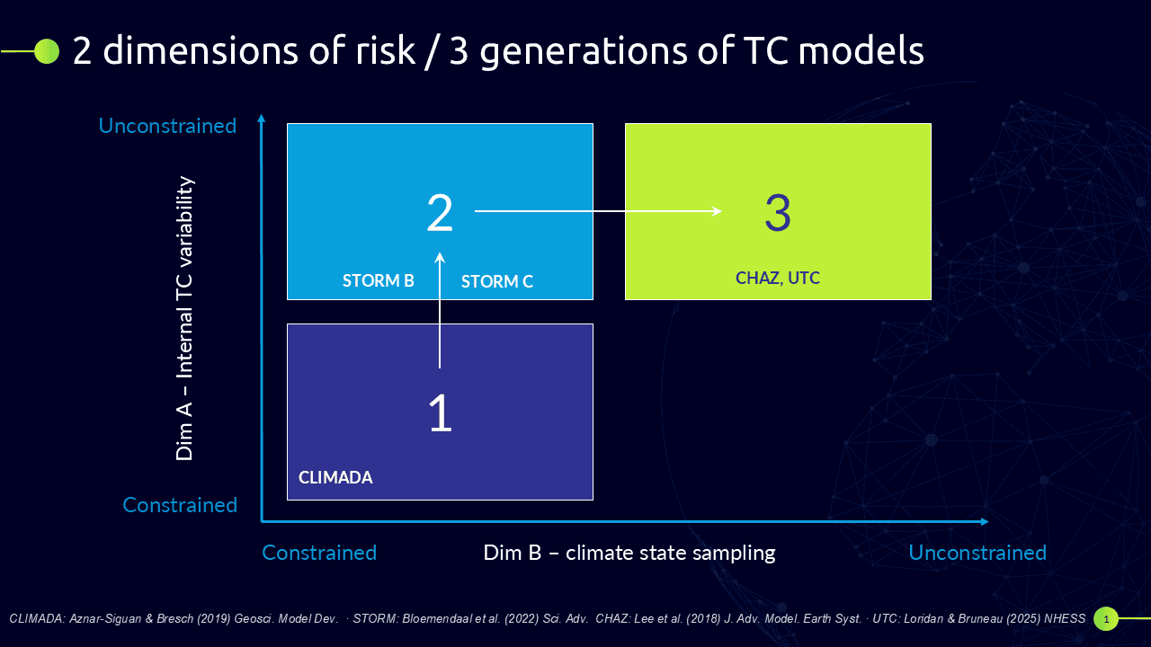
Models shown are published examples of each generation. CLIMADA (Gen 1): Aznar-Siguan & Bresch (2019) Geosci. Model Dev. · STORM (Gen 2): Bloemendaal et al. (2022) Sci. Adv. · CHAZ (Gen 3): Lee et al. (2018) J. Adv. Model. Earth Syst. · UTC (Gen 3): Loridan & Bruneau (2025) NHESS.

The three generations of hurricane risk models 

Historically, models have evolved through this Dim A/B space in three generations:

1. Generation 1 models

Generation 1 models (historical re-samplers, bottom left of the matrix) represent the first attempts at shuffling historical records to create alternative “synthetic events.”

Models in this category typically perturb some aspects of past events (e.g. shifting tracks) but remain shallow in their sampling of dimension A.

They are also designed to represent risk under an average climate representative of what we have experienced (i.e. the period the historical events come from), and are therefore not sampling dimension B.

2. Generation 2 models

Generation 2 models (statistical samplers, top left) are much more sophisticated in their sampling of dimension A, with calibrated components across all key event characteristics (genesis, track, intensity and decay).

However they remain very shallow in how they handle dimension B, with model parameters calibrated to be representative of an average climate over either a past, near-present or future pre-set period.

Importantly, they are statistical models with no direct climate connectivity, and are only aware of the climate state through one-time calibration of their sampling parameters.

3. Generation 3 models

Generation 3 models (climate-connected samplers, top right) build up from generation 2 by introducing gridded climate dataset as live input.

They connect their sampling components directly to the input climate state (e.g. SST, shear, steering and pressure patterns) ensuring synthetic events are being generated with awareness of the climate around them.

Because the climate state is a live input rather than a calibration constraint, they produce a continuous view of risk across dimension B. This allows representation of how large-scale modes like ENSO redistribute tropical cyclone activity between regions, or how global warming is gradually impacting event intensities along the coast. 

The leap from Gen 2 to Gen 3 comes down to one thing: whether the climate state flows through the model continuously, or gets baked in at calibration time and frozen there. That single architectural difference unlocks a set of capabilities that define what these models can and cannot be trusted to tell you.

What continuous climate sampling lets you see

Three capabilities follow from that live climate feed. Each one shows you something a frozen climate state keeps hidden.

Unlock #1: Continuous and granular climate slicing

Without continuous climate-connected sampling, you are only looking through a blurred window onto your hurricane risk, one where the important climate signals have been averaged out and the granularity lost. 

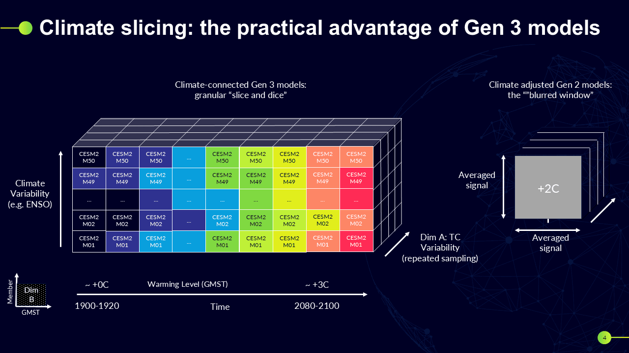
The graphics show the contrast directly: a Gen 3 model deployed continuously across a wide range of climate states (left), versus a Gen 2 model re-calibrated to a single pre-set climate view (right), whether long-term, medium-term, or future.

No matter how a Gen 2 view gets adjusted, the fundamental limitation remains: it can only tell you what risk looks like for a given average climate state.

It can't tell you what risk looks like in an El Niño year with warm basin SSTs, or how warming trends are gradually reshaping the regional distribution of risk along the coast, because the climate is not in the model, only in its calibration.

Gen 3 models unlock those answers. Continuous sampling of Dim B is what turns that blurred window into a sharp image you can zoom in.

Unlock #2: Physics-based regionalisation of risk

When the climate feed is live, risk doesn't just go up or down, it gets physically redistributed.

Gen 3 models are plugged directly into gridded climate data: SSTs, wind shear and steering patterns flow in at every step of the simulation. Genesis likelihood shifts where the ocean is anomalously warm, tracks bend where steering currents change, and intensification accelerates where the thermodynamic environment favours it.

Different parts of the coast respond differently to the same climate state, because the underlying physics play out differently at each location.

The graphic above shows the change in landfall rates along the US coastline for an El Niño year with warm SSTs, compared to the 1980–2025 average.

The signal is not uniform. Some gates see elevated risk, others see suppression. The Gulf and the Northeast move in different directions, not because someone encoded that expectation, but because that's what the physics produces when you feed the actual SSTs, steering and shear patterns into the model chain.

During an El Niño year, positive anomalies of wind shear will tend to reduce risk in the Caribbean and western Gulf; but events that travel north and east of the high shear regions will encounter warm oceans favorable to intensification. This is the granular physics a Gen 3 model captures and translates into a regional coastal view of risk.

That spatial structure is also visible in the tail of the distribution, where physical redistribution matters most.

The graphic below shows how Reask's Unified Tropical Cyclone model translates regional climate anomalies into shifts in hurricane landfall risk, including at return periods where the historical record offers almost no direct guidance.

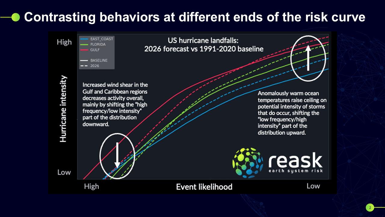
That spatial structure is invisible to a model without climate connectivity. It can only emerge when the climate state flows through genesis, tracks and intensity simultaneously: a signal that emerges through learnt physics rather than pre-imposed calibration.

Unlock #3: Global physics-based generalisation

Gen 2 models are statistical frameworks fitted to historical data. In the North Atlantic, where we have a long period of high quality observations, this works reasonably well. But move to the Bay of Bengal, the South Indian Ocean, or the Arabian Sea, and the historical record thins dramatically.

For a Gen 2 model, thin data means thin calibration. The statistical distributions are poorly constrained, and the model has no way to compensate.

Gen 3 models learn differently. Rather than fitting statistical distributions basin by basin, they learn the physical relationships between climate variables and tropical cyclone behaviour: how SSTs drive potential intensity, how wind shear suppresses development, how circulation patterns steer tracks.

These relationships are universal: a warmer sea surface increases potential intensity whether you are in the Gulf of Mexico or the South Pacific. Because Reask's Unified Tropical Cyclone model is trained globally across all major tropical cyclone basins simultaneously, it applies a globally-learnt physical understanding to local climate signals.

The SSTs and atmospheric conditions of data-sparse basins are well observed, even if their tropical cyclone tracks are not. Utropical cyclone translates those climate signals into risk with physical confidence that no local statistical calibration can matropical cycloneh.

The same global physics also means cross-basin correlations emerge naturally.

When an El Niño suppresses Atlantic activity and simultaneously elevates Eastern Pacific risk, that relationship flows from the same shared climate state driving both responses simultaneously.

For global reinsurers and ILS funds managing multi-basin portfolios, that physically-consistent view of correlated risk is something no collection of independently-calibrated regional models can provide.

Final thoughts: Only Gen 3 models can be trusted for forward-looking risk

Gen 1 and Gen 2 models are, by design, consistent with the historical record. That is the explicit goal of their construction since their statistical components are fitted to reproduce observed tropical cyclone behaviour.

When you validate one of these models against past observations, it will look good, because It was built to.

But here's the problem: today's climate is already measurably different from the period those models were calibrated on.

Atlantic SSTs have reached levels outside the historical envelope. The 2023 season saw MDR temperatures with no precedent in the observational record. The conversion rate from Cat 1 to major hurricane has been trending upward for decades.

A model calibrated to the 1980–2022 average is already describing a climate that no longer exists, and its consistency with past observations offers no assurance that it is capturing what is happening now, let alone what comes next.

Gen 3 models are not calibrated to reproduce historical statistics. They learn the physical relationships between climate variables and tropical cyclone behaviour: how SSTs drive potential intensity, how wind shear suppresses development, how atmospheric circulation steers tracks.

When validated against the historical record, that agreement is genuinely informative: it tells you whether the physics the model has learnt capture real-world tropical cyclone behaviour across the range of observed climate conditions.

When today's SSTs exceed anything in the calibration window, a Gen 3 model can still respond physically, because it has learnt how tropical cyclone behaviour responds to climate conditions, not just what tropical cyclone behaviour looked like in the past.

A Gen 2 model, by contrast, is being asked to describe a climate state it was never built to represent.

Consistency with historical observations is a necessary condition for any model. But it is not sufficient. The right question is not "does your model reproduce the past?," it is rather "does your model understand why the past looked the way it did well enough to be trusted when conditions move beyond it?" 

That distinction is what separates a calibrated statistical description from a physics-based representation of risk. That is why the generational distinction matters, not as a marketing category, but as a question of what you can and cannot trust a model to tell you about a climate that is continuously changing.