Predicting emergency call spikes during and after Hurricane Milton

When hurricanes approach land, emergency services face a critical challenge: how to prepare for the sudden spike in emergency calls. We saw this firsthand during 2024’s Hurricane Milton, where call volumes surged as the storm made landfall. 

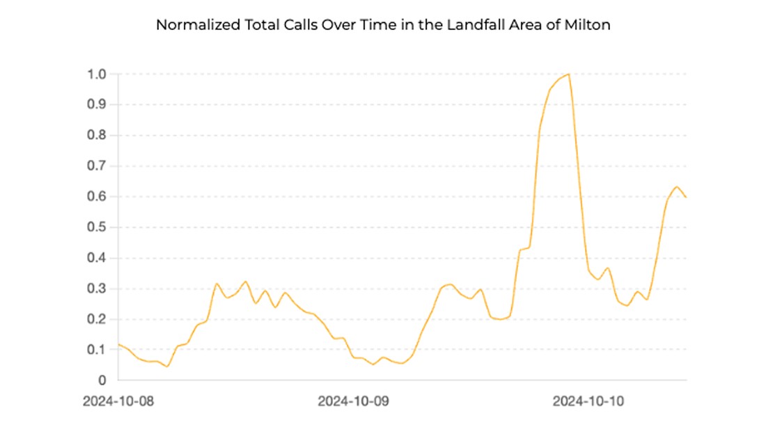
Figure 1. Normalized Total Calls over time in the landfall area of Milton Hurricane.
Data: RapidSOS

Even with strong preparation, call centres can become overwhelmed, leading to delays or calls being routed to distant centres that may not have the local knowledge needed to respond effectively.  

But these spikes in call volume aren’t random. They follow a clear pattern tied to physical hazards like extreme winds, storm surge, and flooding.  

If we can anticipate how these hazards evolve throughout an event, we can give emergency teams a crucial head start, helping them make more informed and efficient staffing and resource allocation decisions. 

That’s where Reask and RapidSOS come in.  

Reask provides both pre-landfall probabilistic hazard forecasts (LiveCyc) and retrospective analyses (Metryc). RapidSOS, a leading platform for integrating safety data, collects detailed emergency call data across the country.  

With this data, we built a predictive model linking storm intensity to emergency call demand, helping translate weather forecasts into operational insight for hurricane-related emergencies. 

In this blog post, we’ll walk through the initial development of that model: how we used historical wind and call data to test our ability to predict emergency call surges during and immediately following Hurricane Milton’s landfall. 

Why we built a call volume prediction model

Our ultimate goal was to accurately predict the timing, magnitude, and spatial pattern of emergency calls during and after a hurricane with up to 72 hours lead time.  

Are we there yet? Not quite. But as you’ll see below, we’re making meaningful progress. 

In this initial study, we tested whether Reask’s retrospective hazard data (Metryc) could be used to accurately estimate emergency call volumes. In other words: if we have our best estimate of what hazards looked like during an event, can we predict the spike in emergency calls? 

It’s a critical first step. The next phase would be to apply the same model to our forward-looking LiveCyc forecasts. If successful, this would enable responders to anticipate call surges days before a storm hits, supporting better resource planning when it matters most.  

The data we used

To build and test the model, we relied on two main data sources:  

1. Metryc – Reask’s historical wind footprint product. It provides “best estimates” along with uncertainty distributions for each ~1 km grid cell around a given event.  

2. RapidSOS emergency call data – Aggregated, anonymized data from a large network of Emergency Call Centres (ECCs), normalized using Uber’s H3 spatial index (at resolution 9).  

These two datasets gave us a detailed view of both the physical storm hazard and the human response, providing the foundation for modelling how the two relate. 

We also pulled in additional contextual data to support the analysis: 

1. Population density from kontur.io, aggregated at H3 (resolution 8). 

2. Storm track information from the International Best Track Archive for Climate Stewardship (IBTrACS). 

Testing the model: What worked and what didn’t

The first step was to examine the spatial distribution of emergency call spikes. If we can’t see a spatial correlation between areas of high winds and areas of high call volume spikes, a predictive model likely won’t perform well either.  

As expected, the patterns aligned. The RapidSOS data showed spikes in call volumes in areas where Metryc estimated the strongest winds.

Figure 2 illustrates this, highlighting the Tampa Bay area as having both the highest wind speeds and most significant surge in emergency calls, measured as the call rate ratio, or CRR, which we define as the ratio of call rate during a 48-hour landfall window to a 3-week pre-event baseline window, accounting for day-of-week patterns. 

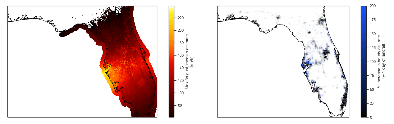
Figure 2. A comparison of maximum 3-second wind gusts (Metryc, left) and CRR (RapidSOS, right). Opacity in the CRR map reflects population density. Data: Reask (left), RapidSOS and kontur.io (right). 

We also visualised the relationship between wind speed and call volume using a bin scatter, grouping locations by wind intensity and comparing average CRR. 

Figure 3 shows how call rates generally increase with stronger winds. At higher wind speeds, where there are few data points, the signal becomes much noisier. All areas outside of the modelled wind footprint (less than 61 km/hr gusts) are grouped at the “0 wind speed” point, which reassuringly shows a CRR of very close to 0.  

In other words, if you are not experiencing hurricane winds, your call volume is unlikely to change. Indeed, it’s not until 100-120 km/hr that we start to see increasing call rates. 

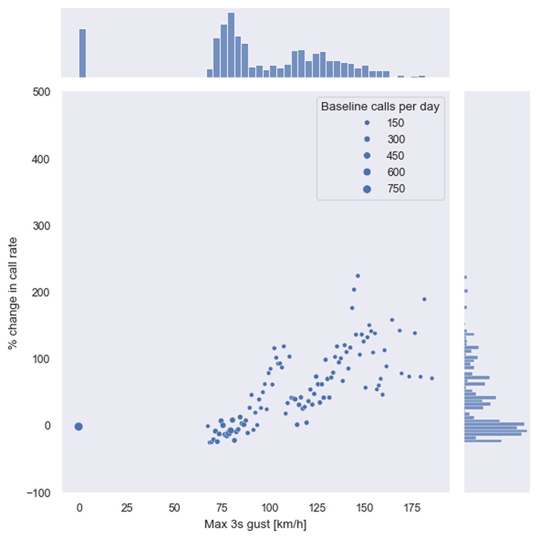
Figure 3. Bin scatter of CRR vs. maximum 3-second wind gusts. Bins with less than 20 baseline calls are excluded to reduce noise. The size of each point is proportional to daily call rate in the baseline period within each bin. Marginal distributions of CRR and wind speed are shown along the plot edges. Data: Reask (wind gust), RapidSOS (CRR). 

This relationship also holds over time. Figure 4 shows this timeseries for all locations receiving <125 and >= 125 km/hr wind gusts during Milton. Locations with higher winds show a clear spike during Milton, while lower wind areas barely register a signal.

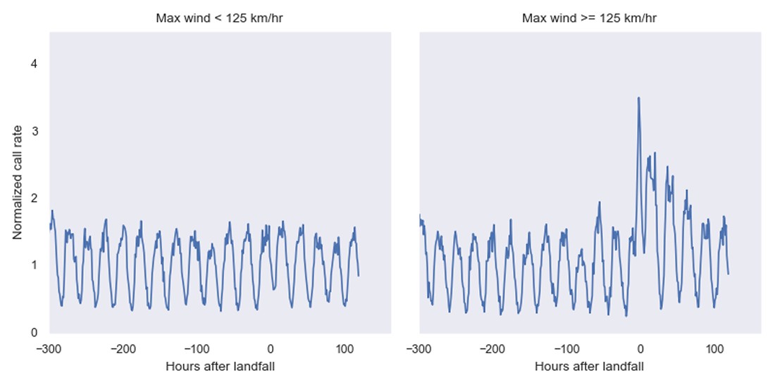
Figure 4. Normalized call rate aggregated across all locations experiencing <125 km/hr maximum wind gusts (left) and all locations experiencing >=125 km/hr maximum wind gusts (right) during Hurricane Milton. Data: RapidSOS (calls), Reask (wind gust). 

Encouraged by these signals, we tested our model’s out-of-sample performance, that is, how well it could predict call volume for a storm it hadn’t seen during training. 

For this, we need to incorporate training data that is not from Hurricane Milton. We trained the model using four past hurricanes: Beryl (2024), Idalia (2023), Ian (2022), and Ida (2021).  

From these events, we built a panel dataset of daily CRR before, during, and after landfall. Our model then employed a pure quadratic fit on daily mean CRR, with fixed daily effects and a time-varying coefficient on wind speed.  

As shown in Figure 5, the strongest relationship between wind and call volume occurs just as the storm hits a location, tapering off in the days that follow. 

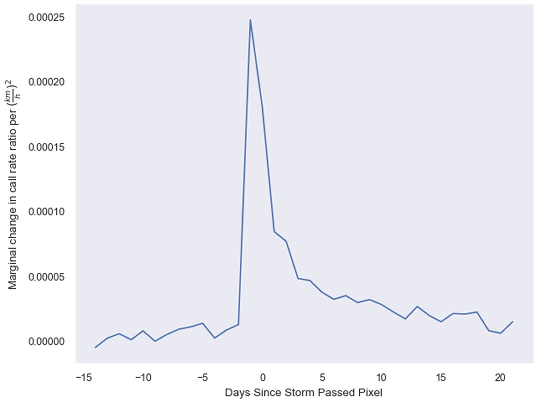
Figure 5. Coefficient on wind speed in the pure quadratic model across 24-hour windows over which we calculate mean CRR. For example, -1 refers to the 24-hour period leading up to the point where a storm passes closest to a given pixel. 

We then applied this model to Milton’s wind data to test its predictive power. Figure 6 shows how the model performed across Florida overall, and within selected counties.

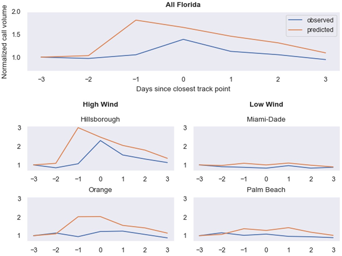
Figure 6. Predicted vs. observed mean daily normalized call volumes across Florida (top) and selected counties (bottom). The counties are chosen among the more populated counties of Florida and are divided between those that experienced high winds from Milton (left) and those that did not (right). 

Overall, we do quite well at predicting call volumes given our fairly simple wind hazard-based model trained on just four historical events. Again, these are out-of-sample predictions, meaning that the model did not see any call volume or wind speed data from Milton during training.  

Across Florida, our estimates slightly overpredict the spike in call volume. This could be due to several factors, for example, the population may have been better prepared than usual, having experienced Hurricane Helene just weeks earlier.  

Our model also tends to anticipate a somewhat earlier response. However, the current daily temporal resolution may exaggerate this timing difference, which is less visible when examining an hourly-based model.  

While better able to predict timing, the hourly model experiences some additional noise that would likely be reduced through training on a more complete set of historical events. 

Looking at individual counties, predictions matched well in three of four high-population areas.  

Low-wind counties showed little change in observed and predicted calls. Hillsborough County (Tampa Bay) had a quite accurate peak call volume prediction, though again, like the full state aggregation, predicts the spike to occur slightly earlier than it does.  

Orange county is an outlier, as this county lay directly in Milton’s path and received substantial wind yet did not see a call volume surge. The outlier can also be seen below in the spatial distribution of CRR in the 48-hour window surrounding the arrival of the storm.  

While the predictions for most counties in Milton’s path appear reasonably accurate, Orange County stands out in the observed data as a noticeably lighter shade of red than its neighbours. It’s unclear why this county did not experience a similar spike in calls, a discrepancy that warrants further investigation.  

There are also no counties where the model predicts a decrease in call volumes. The small drops observed in some areas are likely noise, though it’s possible that certain dynamics cause non-impacted nearby regions to experience lower call volumes during a storm.  

This could be due to public awareness that emergency resources are stretched. If so, this could be a factor worth incorporating into future models. 

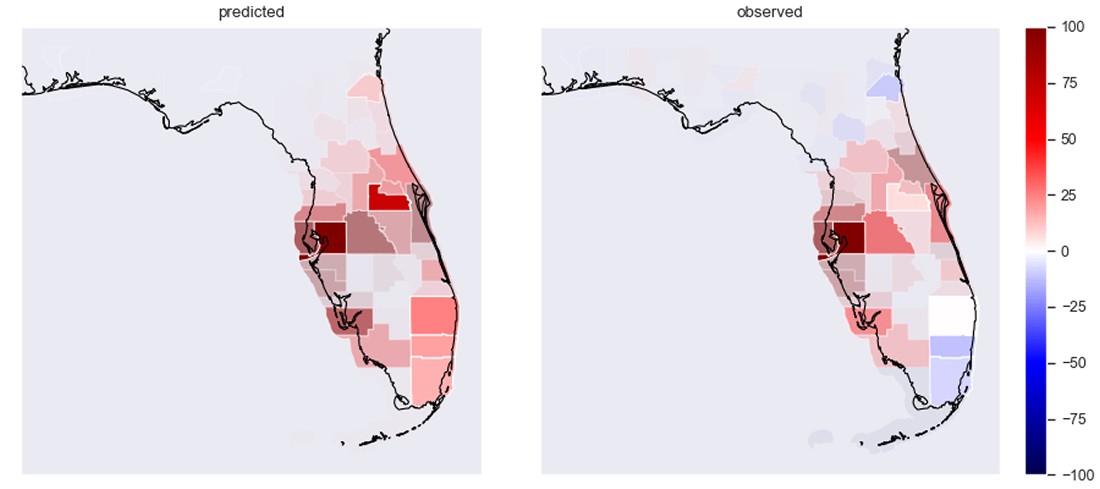
Figure 7. Spatial comparison of predicted and observed CRR during the 48-hour landfall window. Orange county, a notable outlier in the observed call volume surge, is circled. Opacity reflects population size. Data: RapidSOS (observed), Reask + RapidSOS model (predicted). 

What we learned, and future direction

This analysis helped confirm a few key hypotheses:  

• Stronger winds = more emergency calls. Areas with higher wind speeds saw sharper spikes in call volume (Figures 2–4). While wind is a major factor, future models that also include storm surge and inland flooding could offer even more accuracy. 

• Timing matters. Call volumes tend to peak right around landfall, then taper off, though elevated activity often lingers for several days. 

• The model works, despite limited training data. Even with just four past hurricanes in our training set, we were able to predict both the timing and location of call spikes across Florida with reasonable accuracy.  

These early results are encouraging, but perhaps what’s more interesting is the potential direction this work could take. For example, applying the model to LiveCyc, our forward-looking hazard forecast.  

Unlike Metryc (which analyzes past events),  LiveCyc can offer actionable predictions up to 72 hours before landfall, exactly the kind of lead time emergency responders need.  

Expanding the training set and incorporating both coastal and inland flooding estimates could further improve the predictive skill. These additions may also improve the signal-to-noise ratio, potentially enabling higher-resolution outputs (e.g. hourly call volumes instead of daily).  

Finally, this analysis validates a broader approach: using hazard data to forecast a wide range of hurricane impacts beyond insured losses.  

Power outages, business disruptions, financial market impacts, and a variety of other impacts are all likely predictable with the type of spatially and temporally granular wind and flood hazard data that Reask can generate in both forecast and hindcast contexts.   

Even longer-term effects, such as hurricanes’ impact on mortality rates up to a decade later, may also be predictable. 

There are many ways in which these powerful events impact our society, and Reask is developing the tools to better predict and ultimately respond to them.  

You can explore the code used to generate this analysis on GitHub. Although the underlying Reask and RapidSOS data aren’t publicly accessible, the notebook outlines the full approach for those interested in the methodology.  

If you would like to discuss access to either of these datasets, please reach out to contact@reask.earth or visit rapidsos.com/contact, respectively.